Decentralized Online Learning of Stackelberg Equilibrium in General-Sum Leader-Controller Markov Games

Currently Under Review

A brief game theory supplement

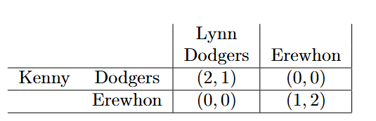
I want to go watch the Dodgers game, but Lynn really wants to go to Erewhon. However, if we both go to the Dodgers game, Lynn will be less happy than me, and similarly, if we both go to Erewhon, I’ll be less happy than Lynn. Yet we still want to go somewhere together; not going together is worse than going together anywhere.

Such a simple interaction between Lynn and I is a case of the “Battle of the Sexes”, a classic example from the field of game theory, which studies how individuals make decisions when their outcomes depend on the decisions of others as well. Games can come in many different forms, yet each one has the following standard “ingredients”:

1. The players. Who are the individuals in the game interacting with each other? For example, Lynn and I.
2. The actions. What can each player do? For example, either one of us can either go to the Dodgers game or Erewhon.
3. The information. What does each player know? For example, do I know Lynn has already decided to go to Erewhon?
4. The preferences. Which outcomes do the players prefer over others? For example, I prefer both of us going to the Dodgers game versus both of us going to Erewhon, but Lynn is the opposite. Each outcome can be valued through the payoff the player receives.

With these ingredients, we can express this game as a “payoff matrix”, where the rows correspond to one player’s actions (me) and the columns correspond to the other player’s actions (Lynn). The left value in each cell corresponds to the payoff I receive if we take those respective actions, and the right value corresponds to the payoff Lynn receives. So I receive more payoff than Lynn if we both go to Dodgers, while vice versa if we both go to Erewhon.

image.png

Players thus decide on strategies or policies, which dictate what actions they should play. These could be pure strategies (e.g. I simply choose “Dodgers”) or mixed strategies (e.g. I choose “Dodgers” 50% of the time and “Erewhon” the other 50%).

As with any other problem, we need a solution concept. In games, economists often look for equilibria, which roughly speaking, are points of “stability”. The most famous is the Nash equilibrium, which is defined as a set of strategies where no player benefits from a unilateral deviation.

This is best seen through an example of a Nash equilibrium in the game above. Consider the pure strategy profile (Dodgers, Dodgers). Consider the unilateral deviations, where only one player switches their action. If I choose Erewhon, my payoff decreases from \(2\) to \(0\), so I would not benefit. Similarly, Lynn would not benefit by switching to Erewhon, as her payoff would decrease from \(1\) to \(0\). Thus, (Dodgers, Dodgers) consistutes a pure-strategy Nash equilibrium.

For a similar reason, (Erewhon, Erewhon) is also a Nash equilibrium. Suprisingly, there is in fact a third Nash equilibrium consisting of mixed strategies, where neither player’s expected payoff increases from a unilateral deviation. This is not really relevant for this paper, but still a very important concept within game theory! Try to find it as a challenge.

Stackelberg/sequential games

The Stackelberg model is a special kind of game-theoretic model that situates players within a “leader-follower” dynamic. For example, firm \(F\) could be choosing to enter a market by producing some nonzero amount of product. However, if there is already firm \(L\) in the market, they have the power of choosing how much to produce first. If firm \(L\) is strategic, they could produce a larger than normal quantity, lowering the market price of the product, which deincentivizes the entry of firm \(F\) and eliminates competition. See here for a worked out theoretical example.

More generally, a sequential game is one where one player(s) (the “leader(s)”) has the ability to move first, then the other player(s) (the “follower(s)”) observes what the leader takes and then takes their action. When deciding strategies, the follower’s strategy is now conditional on that of the leader. A strategy for the follower thus needs an action for each potential leader action. For example, if Lynn is the leader, one strategy would be to play “Erewhon”, while I as the follower could take the strategy {Erewhon | Erewhon, Dodgers | Dodgers}, where \(a | b\) means I choose action \(a\) if Lynn chooses action \(b\).

In the “Battle of the Sexes” example, if Lynn is the leader, she has the ability to choose “Erewhon” first, and so I, trying to maximize my payoff, choose “Erewhon” as well as my best-response. If she chose “Dodgers”, then my best-response would be “Dodgers”. Lynn, realizing this, uses backwards induction and determines that she should choose “Erewhon” to maximize her payoff.

In this sense, (Erewhon, {Erewhon | Erewhon, Dodgers | Dodgers}) constitutes a Nash equilibrium for this sequential game. Similarly, (Erewhon, {Erewhon|Erewhon, Erewhon|Dodgers}) would also be an equilibrium, since Lynn would not want to switch to Dodgers, and I would not want to change my strategy conditional on Lynn playing Erewhon either.

Interestingly, (Dodgers, {Dodgers | Erewhon, Dodgers | Dodgers}) is also an equilibrium! (Can either of us benefit from a unilateral deviation of our strategy?) But Lynn should have the intuitive advantage of choosing Erewhon first. What’s happening here is that I am essentially “threatening” Lynn to play Dodgers by saying I will still choose Dodgers if she chooses Erewhon, even if it’s worse off for me. Some game theorists don’t really find this solution intuitive (of course, Lynn would see through my bluff immediately), so there is an alternate equilibrium concept in sequential games known as a subgame-perfect Nash equilibrium that eliminates these so called “non-credible threats”.

That’s been a brief background of some of the game theory background you need for this paper (which in essence, is still a reinforcement learning paper). I’d like to end this section with some remarks:

• One key note to mention here is in these settings, players had full information about their own and other players’ payoffs. When we adapt this setting into a learning problem (i.e. the crux of this paper), we assume these are unknown to the players, and they have to learn the payoffs through sampling. This is one key difference between how economists and learning researchers can study games.
• While we can study the existence and uniqueness of equilibria, game theory doesn’t really tell us which equilibrium the game will settle to, nor does it tell us how these systems evolve to reach these equilibria. Again, equilibria are just points of “stability”. In the simulatenous game, (Dodgers, Dodgers) is a better equilibrium for me, but (Erewhon, Erewhon) is better for Lynn. Which one will the game settle to?
  • However, in algorithmic game theory, where this economic intuition is less emphasized and we just try to learn and converge to equilibria (which are usually unique in a game), this learning process is more clear.

Learning Equilibrium in Stackelberg Markov Games

At last we reach the reinforcement learning theory. In algorithmic game theory, our goal is to develop algorithms for some game that dictate what policies the players take, such that over time, they minimize players’ regret and/or learn and converge to some equilibrium within some degree of approximation. For this paper, we adapt the Stackelberg game model into a two-player Markov decision process (MDP), where the rewards and transition dynamics are dictated by the joint actions of both players. For a background to MDPs, I recommend checking out this blog, where I briefly introduce the finite, tabular, single-agent MDP. The key distinctions here are that in any given state, the leader first takes an action, then the follower sees this action and responds with an action of their own. Both the leader and follower have the own respective payoff/loss functions which depend on both players’ actions. Neither player knows their own loss functions; they can only observe the actions being played and the noisy losses they receive.

Leader-controller Markov games and game reward structures

For this Markov game in particular, we impose a leader-controller assumption, where the transition dynamics only depend on the action the leader takes. Allow me to discuss why such an assumption is important.

As we’ve seen before, in a game, the rewards of one player depend on the very potentially arbitrary actions of the other player. While the rewards for some joint-action can be constant or come from some fixed distribution, this dependence on other player’s actions inherently makes the reward observations somewhat arbitrary, taken from the reference from of a single player. Thus, games ride this weird “middle-ground” between stochastic and adversarial-based rewards. It also should then be no surprise that in standard bandit games, algorithms designed to converge to Nash equilibria use the exponential weights algorithm for each player, an algorithm designed for regret minimization in adversarial environments.

When we move to Markov games however, both players now can affect the transition dynamics, making the transitions potentially arbitrary from the reference frame of one player. In this same blog, we deal with the corrupted setting where the transitions are potentially arbitrary. Importantly, in these settings, if the level of corruption in the transitions is high, players can be doomed to experience linear regret.

Thus, by suppressing the transitions’ dependence on the follower, we make both regret minimization and equilibrium learning for the players feasible in Markov games.

What’s Stackelberg equilibrium in Markov games?

Recall that Stackelberg equilibrium constitutes both player’s choosing policies that best-respond to the other player.

For the follower, since their actions no longer influence the transitions, their environment is dictated by what state they are in and what action the leader takes. In this sense, their learning problem reduces to parallel stochastic bandits for each state, leader-action tuple they can encounter. We make the standard assumption that the follower’s best-response to any leader action is unique, and thus define the follower’s optimal or , \(\pi^f_\star\), to be that for which for each state-leader action pair \((s,a)\),

\[\begin{equation} \pi^f_\star(s,a) := \underset{\pi^f}{\arg\min} \ \mathbb{E}_{k \sim \pi^f(\cdot|s,a)}\left[l^f(s,a, k)\right]. \end{equation}\]

For the leader, their learning problem is now akin to an adversarial MDP. Given a leader loss function \(\ell\), leader policy \(\pi\), and follower policy \(\pi^f\), we can define the leader’s expected sum of losses for the remainder of an episode starting from state \(s_{h'}\) in some layer \(h'\), \(h'=0, 1, \ldots, H-1\), as: \[\begin{equation} V^{\pi, \pi^f}(s_{h'};\ell) := \mathbb{E}_{\substack{a_h \sim \pi(\cdot|s_{h}), \\ k_h \sim \pi^f(\cdot|a_h, s_h), \\ s_{h+1} \sim P(\cdot |s_{h}, a_h)}} \left[\sum_{h=h'}^{H-1} \ell(s_{h},a_h, k_h) \right] \end{equation}\] where \(V\) is called the leader’s state value function or \(V\)-value function, given the leader follows policy \(\pi\) and the follower follows policy \(\pi^f\).

Thus, we say \((\pi_\star, \pi^f_\star)\) constitutes a Stackelberg equilibrium (SE) if the leader policy \(\pi_\star\) is in \(\arg\min_\pi V^{\pi, \pi^f_\star}(s)\) for all states \(s\). In particular, for the \(T\)-episodic Stackelberg Markov game, we say that \(\pi_T\) is an if for all \(s \in \mathcal{S}\), the value functions at state \(s\) under \((\pi_T, \pi^f_\star)\) and some SE \((\pi_{\star}, \pi^f_\star)\) are \(\varepsilon\) apart, i.e. \(V^{\pi_T, \pi^f_\star}(s) \leq V^{\pi_\star, \pi^f_\star}(s) + \varepsilon\).

Our goal is to develop algorithms, in particular, decentralized algorithms, that provably allow the players to converge to a Stackelberg equilibrium while minimizing individual player regret.

Our contribution

We frame learning Stackelberg equilibrium as a reinforcement learning problem. Namely, we first define MDP Stackelberg regret as:

\[\begin{equation}\label{eq: stackelberg_regret} R_{\text{Stack}}(T) := \sum_{t=1}^T V^{\pi_t, \pi^f_\star}(s_0; \ell) - \min_{\pi} \sum_{t=1}^T V^{\pi, \pi^f_\star}(s_0; \ell). \end{equation}\]

The second term of \(R_{\text{Stack}}(T)\) are the total leader losses in SE, and so we see algorithms whose MDP Stackelberg regret scale sub-linearly with \(T\) converge to a SE. Note that in the first term of \(R_{\text{Stack}}(T)\), the follower’s best-response policy is fixed as well, which differentiates Stackelberg regret analysis from that of a traditional single-agent adversarial MDP, where the first term would instead be the expected incurred losses of the leader during play (with the follower playing \(\{\pi^f_t\}_{1\leq t \leq T}\)). Stackelberg regret thus intuitively incorporates the “learning capacity” of the regret-minimizing follower; indeed, if \(\pi^f_t \neq \pi^f_\star\) for many \(t\), this may prevent the leader from adequately learning \(\pi_\star\) themselves, leading to increased Stackelberg regret.

In our paper, we introduce a decentralized policy optimization algorithm for Stackelberg equilibrium learning. The crux of our algorithm lies in the rather-intuitive combination of no-regret algorithms: an Upper Confidence Bound-based algorithm for the follower with a no-regret adversarial MDP policy optimization scheme inspired by Luo et al. 2021 for the leader, which lends itself to high computational efficiency and strong empirical performance.

The policy optimization-based Algorithm 1 of Luo et al. 2021 achieves \(\widetilde{\mathcal{O}}(\sqrt{T})\) regret in adversarial MDPs by computing stochastic policies using exponential weight updates on \(Q\)-value estimates, \(\widehat{Q}_t\), for each state-action pair each round. These estimates are built using an estimated model where optimistic state-action occupancy measures under some policy \(\pi_t\) (\(\overline{q}_t(s,a)\)) are computed by taking the maximum over transition functions within a confidence set (see \(\texttt{COMP-UOB}\), Algorithm 3 of Jin et al. 2020. This confidence set is carefully constructed around an empirical estimate of the transition to contain the true transition with high probability and is updated when the number of visits to some state-leader action pair doubles. The period between two updates is called an epoch, and the transition confidence set in epoch \(k\) is denoted \(\mathcal{P}_k\). We remark that because of Assumption \(\ref{assumption:leader}\), the leader is able to estimate the from their own actions taken in this manner. Furthermore, to address the global exploration limitations of policy optimization, Luo et al.  also introduce dilated bonuses \(B_t\) subtracted from the \(Q\)-estimates that utilize the high-probability occupancy bounds to encourage exploration of rarely visited states and actions.

On the myopically-rational follower’s side, learning \(\pi^f_\star\) amounts to identifying the unique best-response \(\pi^f_\star(s,a) \in \mathcal{K}\) for each state-leader action pair \((s, a)\). The follower can thus run \(SA\) UCB algorithms, treating each \((s, a)\) as an independent environment, and achieve optimal regret for sufficiently large \(T\). For a given round \(t\) and for each \((s,a)\) visited, the follower chooses \(\pi^f_t(s,a) \in \arg\min_k \text{UCB}_{(s,a)}(k)\), where for all \((s,a,k), \text{UCB}_{(s,a)}(k)\) is computed by: \[ \begin{multline}\label{eq:followerucb} \text{UCB}_{(s,a)}(k) := \widehat{l}^f_{s,a,k}(t-1) - \sqrt{\frac{6\log n_{(s,a)}(t-1)}{n^f_k(n_{(s,a)}(t-1))}} \end{multline} \] where \(n_{(s,a)}(t-1)\) is the number of times state-leader action \((s,a)\) is visited up to time \(t\), \(n^f_k(x)\) is the number of times the follower takes response \(k\) across \(x\) instances of some state-leader action \((s,a)\), and \(\widehat{l}^f_{s,a,k}(t-1)\) is the empirical mean loss estimate up to round \(t\) from taking \(k\) in \((s,a)\) updated as follows: \[ \begin{multline} \widehat{l}^f_{s,a,k}(t) = \frac{1}{n^f_k(n_{(s,a)}(t))}\Biggl( \widehat{l}^f_{s,a,k}(t-1)\cdot n^f_k(n_{(s,a)}(t-1)) \\ + \sum_{h=0}^{H-1} \ell^f(s_{t,h}, a_{t,h}, k_{t,h})\cdot \mathbb{I}\left[(s,a,k) = (s_{t,h},a_{t,h},k_{t,h})\right]\Biggr). \end{multline} \] The UCB is set to \(-\infty\) if \(n^f_k(n_{(s,a)}(t-1)) = 0\). We remark that because of the partitioned state-space, any \((s,a)\) can be visited a maximum of one time per episode.

*\(\alpha\)-Exploration, Estimators, and Bonuses} Our first novel contribution needed to adapt this framework for minimization is using the policy \(\widetilde{\pi}_t\), which incorporates a fixed explicit exploration parameter \(\alpha\) into the leader’s policy taken from exponential weights, \(\pi_t\). This ensures that in any state, the probability of selecting any action \(a\) is at least \(\alpha/A\). This extends from the exploration mechanism in Yu et al.  for the bandit setting, ensuring that the leader plays all actions often enough for the follower to reliably learn its best response. Note that such an explicit exploration technique can only be run on the level of the action set, not of the states. Without Assumption \(\ref{assumption:leader}\), a state could hypothetically only be reached via one trajectory, resulting in, at worst, an exponential in \(H\) dependency on the probability that some \((s,a)\) is reached. Therefore, Assumption \(\ref{assumption:leader}\) is essential for making Stackelberg equilibrium learning tractable in the decentralized setting by ensuring best-response identification for the follower without coordination assumptions. Choosing \(\alpha\) to be on the order of \(\mathcal{O}(T^{-1/4})\) balances the sampling needs of the follower with regret-minimization of the leader, guaranteeing sublinear MDP Stackelberg regret as highlighted in Theorem \(\ref{theorem:regret}\).

However, since our loss feedback now comes from \(\widetilde{\pi}_t\), we diverge from Luo et al.  by instead constructing \(Q\)-value estimates for \(Q_t^{\widetilde{\pi}_t}\). Formally, let \(\{s_{t,h}, a_{t,h}, k_{t,h}, \ell(s_{t,h}, a_{t,h}, k_{t,h})\}_{h=0}^{H}\) be the trajectory received by the leader on episode \(t\) taking policy \(\widetilde{\pi}_t\) and let \(k\) be the current epoch. For \(h \in \{0, 1, \ldots , H\}\), \((s,a) \in \mathcal{S}_h \times \mathcal{A}\), we compute: \[\begin{equation}\label{eq:qestimator} \widehat{Q}_t(s,a) := \frac{L_{t,h}}{\bar{q}_t(s,a) + \gamma}\mathbb{I}_t(s,a) \end{equation}\] where \(L_{t,h} := \sum_{i=h}^{H} \ell(s_{i,h}, a_{i,h}, k_{i,h})\), \(\bar{q}_t(s,a) := \max_{\widehat{P}\in \mathcal{P}_k} q^{\widehat{P}, \widetilde{\pi}_t}(s,a)\), and \(\mathbb{I}_t(s,a) := \mathbb{I}[s_{t,h} = s, a_{t,h} = a]\).

Importantly, the upper occupancy bound \(\overline{q}_t(s,a)\) is computed under the policy \(\widetilde{\pi}_t\) to make \(\widehat{Q}\) an appropriate optimistic under-estimator for \(Q^{\widetilde{\pi}_t}\).

Our last algorithmic novelty is making a subtle adjustment to the dilated bonuses of Luo et al. . Formally, let \(k\) be the current epoch and we compute for all \((s,a) \in \mathcal{S} \times \mathcal{A}\): \[\begin{equation}\label{eq:bonuses1} b_t(s) = \mathbb{E}_{a \sim \pi_t(\cdot \mid s)} \left[ \frac{3 \gamma H + H \big( \bar{q}_t(s,a) - \underline{q}_t(s,a) \big)} {\bar{q}_t(s,a) + \gamma} \right] \end{equation}\] \[\begin{equation}\label{eq:bonuses2}\begin{split} &B_t(s,a) = b_t(s) \\ &+ \left( 1 + \frac{1}{H} \right) \max_{\widehat{P} \in \mathcal{P}_k} \mathbb{E}_{s' \sim \widehat{P}(\cdot \mid s,a)} \mathbb{E}_{a' \sim \pi_t(\cdot \mid s')} \big[ B_t(s',a') \big] \end{split} \end{equation}\] where \(\underline{q}_t(s,a) = \min_{\widehat{P} \in \mathcal{P}_k} q^{\widehat{P}, \widetilde{\pi}_t}(s,a), B_t(s_H,a) = 0\) for all \(a\).

Notice how the upper and lower occupancy bounds are computed with respect to the actual policy taken, \(\widetilde{\pi}_t\), but the is taken with respect to the policy drawn from exponential weights, \(\pi_t\). This subtle change is crucial for bounding the regret of the leader’s learning process, ensuring that we can use the recursive process in Lemma 3.1 of Luo et al.  to control the regret incurred from bonuses. With these additions, we state the following result.

Notably, Theorem \(\ref{theorem:regret}\) shows that Algorithm \(\ref{algo:UOBREPSUCB}\) establishes the first sublinear Stackelberg regret guarantee for decentralized Stackelberg Markov games setting on the order of \(\mathcal{O}(T^{3/4})\) with high probability, extending current guarantees in the decentralized bandit setting while preserving high computational efficiency with policy optimization methods. Full details on computing the transition confidence set \(\mathcal{P}_k\), occupancy bounds, and other algorithmic details can be found in Appendix \(\ref{appendix:UOBREPS}\). The full proof of Theorem \(\ref{theorem:regret}\) is in Appendix \(\ref{proof:regret}\), and the key details of the analysis are highlighted in Section \(\ref{sec:analysis}\).

As a corrollary to Theorem \(\ref{theorem:regret}\), we show how the players can learn an \(\varepsilon\)-approximate Stackelberg equilibrium in the \(T\)-episodic SLSF Stackelberg MDP setting if both employ Algorithm \(\ref{algo:UOBREPSUCB}\), at a \(\widetilde{\mathcal{O}}\left(T^{-\frac{1}{4}}\right)\) rate. To see this, define the \(\bar{\pi}\) given by: \[\begin{equation} \bar{\pi}(\cdot|s) = \frac{1}{T}\sum_{t=1}^T\widetilde{\pi}_t(\cdot|s). \end{equation}\] for all \(s \in \mathcal{S}\). After \(T\) episodes, the leader can implement \(\bar{\pi}\) (with the follower best-responding) by sampling \(t\) uniformly from \(\{1, \dots, T\}\) at each state and then sampling \(a \sim \widetilde{\pi}_{t}(\cdot | s)\). This leads to the following theorem, the proof of which is found in Appendix \(\ref{proof:equilibrium}\).

%

% Here, we demonstrate the flexibility of our Stackelberg regret analysis through incorporating alternative sublinear regret algorithms for Markov games that also allow the players to converge to Stackelberg equilibrium, which extends results of equilibrium convergence in bandit games . In particular, for the leader, the best known regret guarantee in the adversarial MDP setting is that of the algorithm which achieves \(\widetilde{\mathcal{O}}\left(HS\sqrt{AT}\right)\) regret, albeit more inefficiently than policy optimization as it performs global convex optimization over all state occupancy measures using relative entropy. In Algorithm \(\ref{algo:UOBREPSUCB2}\), we substitute in \(\textsc{UOB-REPS}\) for the leader, which improves the Stackelberg equilibrium learning guarantee’s dependence on \(H\):

% \begin{theorem} % In the \(T\)-episodic Stackelberg Markov game setting (Section \(\ref{sec:preliminary}\)), if the leader and follower apply Algorithm \(\ref{algo:UOBREPSUCB2}\) and set \(\alpha = \mathcal{O}(H^{-1} SA^{\frac{2}{3}}(\log A)^{\frac{1}{3}} T^{-\frac{1}{3}})\), with probability at least \(1-\mathcal{O}(\delta)\), the Stackelberg regret is bounded as: % \[ % R_{\text{Stack}}(T) \leq \widetilde{\mathcal{O}}\left(\frac{H^2SA^{\frac{4}{3}}KT^{\frac{1}{3}}}{\beta\varepsilon^2} + H^2SA^{\frac{2}{3}}T^{\frac{2}{3}} % \right) % \] % where \(\widetilde{\mathcal{O}}\) hides logarithmic dependencies.

% Furthermore, with probability at least \(1-\mathcal{O}(\delta)\), the time-averaged policy \(\bar{\pi}\) constitutes a \(\varepsilon_T\)-SE where \(\varepsilon_T = \widetilde{\mathcal{O}}\left(\frac{H^3SA^{\frac{4}{3}}KT^{-\frac{2}{3}}}{\beta\varepsilon^2} + H^3 SA^{\frac{2}{3}}T^{-\frac{1}{3}} % \right)\). % \end{theorem}

% The pseudocode for Algorithm \(\ref{algo:UOBREPSUCB2}\) is in Appendix \(\ref{appendix:UOBREPS}\) and the proof of Theorem \(\ref{theorem:UOBREPS2}\) is in Appendix \(\ref{proof:regret2}\).

We present a high-level overview of the proof of our main result, Theorem \(\ref{theorem:regret}\), here and defer the details to Appendix \(\ref{proof:regret}\). We first decompose \(R_\text{Stack}(T)\) into the terms: \[\begin{align*} R_{\text{Stack}}(T) &=\sum_{t=1}^T \left(V^{\pi_t, \pi^f_*}\left(s_0\right) - V^{\pi_*, \pi^f_*}(s_0)\right) \\ & =\underbrace{\sum_{t=1}^T \left(V^{\pi_t, \pi^f_*}\left(s_0\right)-V^{\pi_t, \pi^f_t}\left(s_0\right)\right)}_{\text{(Term I)}}\\ &+\underbrace{\sum_{t=1}^T \left(V^{\pi_t, \pi^f_t}\left(s_0\right)-V^{\pi_*, \pi^f_t}\left(s_0\right)\right)}_{\text{(Term II)}}\\ &+\underbrace{\sum_{t=1}^T \left(V^{\pi_*, \pi^f_t}\left(s_0\right)- V^{\pi_*, \pi^f_*}\left(s_0\right)\right)}_{\text{(Term III)}} \end{align*}\] Terms I and III capture the learning of the follower. We first bound the empirical values of these terms by the number of times the follower does not best-respond to the state-leader actions visited, which are small by 1) standard UCB analysis on the number of pulls needed to learn a best-response given any state-leader action environment, and 2) the explicit \(\alpha\) exploration parameter, set to \(\mathcal{O}(T^{-\frac{1}{4}})\), which allows each state-leader action to be visited enough times across so that the follower can adequately learn the best-response. Combining this with Azuma’s concentration inequality to bound the expected values (see Lemmas \(\ref{lemma:i}\) and \(\ref{lemma:iii}\)), we get that \(1-\mathcal{O}(\delta)\) probability: \[\begin{align*} &\text{Term I}\leq \\ &\mathcal{O}\left(SAK\left(\frac{\log T}{\varepsilon^2}+\log\left(\frac{SAK}{\delta}\right)\right)+H\sqrt{T\log\left(\frac{1}{\delta}\right)}\right) \\ &\text{Term III} \leq \\ &\mathcal{O}\Biggl(H^2S^{\frac{1}{2}}AKT^{\frac{1}{4}}\frac{\log(1/\delta)}{\beta} \cdot \left(\frac{\log T}{\varepsilon^2}+\log\left(\frac{SAK}{\delta}\right)\right) \\ &\quad+ H\sqrt{T\log\left(\frac{1}{\delta}\right)}\Biggr). \end{align*}\]

Term II draws back to the motivation in using no-regret adversarial MDP algorithms for the leader, and where we draw on policy optimization techniques in Luo et al. . We first suppress the value functions’ dependence on the follower’s policies \((\pi^f_t)\) by treating the leader’s losses as adversarial, thus bounding Term II by the regret of a single-agent adversarial MDP. From here, the challenge lies in bounding the additional regret incurred by the \(\alpha\) exploration taken by \(\widetilde{\pi}_t\), rather than using the unmodified \(\pi_t\). We use the well-known performance difference lemma to bound Term II by: \[ \text{Term II} \leq \sum_{s\in\mathcal{S}} q^{\pi_\star}(s) \sum_{t=1}^T \sum_{a \in \mathcal{A}} \left(\widetilde{\pi}_t(a| s)-\pi_\star(a| s)\right) Q_t^{\widetilde{\pi}_t}(s,a) \] where \(q^\pi(s)\) is the probability of visiting state \(s\) following policy \(\pi\) and \(Q_t^\pi\) is the (hypothetical) adversarial \(Q\)-value function that has suppressed the follower’s policies. Using the definition of \(\widetilde{\pi}\), we can further bound: \[\begin{align*} &\text{Term II}\leq \\ & \underbrace{\sum_{s\in\mathcal{S}} q^{\pi_\star}(s) \sum_{t=1}^T \sum_{a \in \mathcal{A}} \left(\pi_t(a| s)-\pi_\star(a| s)\right) Q_t^{\widetilde{\pi}_t}(s,a)}_{(\star)} + \mathcal{O}(\alpha TH^2). \end{align*}\] Next, to bound \((\star)\), we aim to invoke Lemma 3.1 from Luo et al.  (restated in Lemma \(\ref{lemma:eq3.1}\)), which holds due to our modification of the dilated bonuses—namely, the expectations with respect to \(\pi_t\). To this end, we perform the following decomposition: \[\begin{align*} &\sum_{s\in\mathcal{S}} q^{\pi^\star}(s) \sum_{t=1}^{T} \left\langle\pi_t(\cdot| s) - \pi^\star(\cdot| s), Q_t^{\widetilde{\pi}_t}(s,\cdot) - B_t(s,\cdot)\right\rangle \\ &\underbrace{\leq \sum_{s\in\mathcal{S}} q^{\pi^\star}(s) \sum_{t=1}^{T} \left\langle\pi_t(\cdot| s), Q_t^{\widetilde{\pi}_t}(s,\cdot) - \widehat{Q}_t(s, \cdot)\right\rangle}_{\text{BIAS-1}} \\ &+\underbrace{ \sum_{s\in\mathcal{S}} q^{\pi^\star}(s) \sum_{t=1}^{T} \left\langle \pi^\star(\cdot| s), \widehat{Q}_t(s, \cdot) - Q_t^{\widetilde{\pi}_t}(s,\cdot)\right\rangle}_{\text{BIAS-2}} \\ &+ \underbrace{\sum_{s\in\mathcal{S}} q^{\pi_\star}(s) \sum_{t=1}^T \left\langle \pi_t(\cdot| s)-\pi_\star(\cdot| s), \widehat{Q}_t(s,\cdot) - B_t(s,\cdot)\right).}_{\text{REG-TERM}} \end{align*}\]

BIAS-1 and BIAS-2 can be bounded using identical techniques to Lemmas C.1 and C.2 from Luo et al. , due to the fact that we constructed \(\widehat{Q}_t\) to be good optimistic estimators of \(Q_t^{\widetilde{\pi}_t}\). Additionally, since the unmodified \(\pi_t\) is drawn from the exponential weights algorithm with \(\widehat{Q}_t - B_t\) as loss vectors, we can apply the well-known regret bound (restated in Lemma \(\ref{lemma:expweights}\)) and follow through with the rest of the reasoning in Lemma C.3 of Luo et al.  to bound REG-TERM. After verifying a few details, applying Lemma \(\ref{lemma:eq3.1}\) thus allows us to bound with high probability: \[\begin{align*} &\text{Term II} \leq \tilde{\mathcal O}\!\,\Biggl(\frac{H}{\eta} + \alpha TH^2 +\\ &\sum_{t=1}^{T} \sum_{s,a} q^{\widehat P_t,\pi_t}(s)\,\pi_t(a|s)\, \frac{\gamma HA + HA(\overline{q}_t(s,a) - \underline{q}_t(s,a))} {\left( \bar q_t(s) + \gamma\right)\cdot \alpha} \Biggr), \end{align*}\] where we used the lower bound \(\alpha/A \leq \widetilde{\pi}_t(a|s)\) in the denominator of the bonus term. The \(\overline{q}_t - \underline{q}_t\) term is well-bounded due to our shrinking confidence set (see Lemma 4 from Jin et al. ). The last challenge is comparing the occupancy measures \(q^{\widehat P_t,\pi_t}(s)\) and \(\bar q_t(s)\), the latter of which is under \(\widetilde{\pi}_t\). Using the inequality \(\pi_t \leq \frac{\widetilde{\pi}_t}{1-\alpha}\) and backwards induction, we can show (in Lemma \(\ref{lem:occ_domination}\)) that for any \(s\), \(q^{\widehat{P}_t,\pi_t}(s)\) is upper bounded by \(q^{\widehat{P}_t,\widetilde{\pi}_t}(s)\) times a factor of just \((1-\alpha)^{-H}\), which is small for large \(T\) with our choice of \(\alpha\). This resolution of the policy mismatch allows us to finish the proof techniques of Luo et al. , and we show with Lemma \(\ref{lemma:ii}\) that by balancing our choice of \(\alpha\) and \(\eta\), we have that with probability at least \(1-\mathcal{O}(\delta)\),: \[ \text{Term II} \leq \widetilde{O}\left(H^4 + H^3SA^{\frac{1}{2}}T^{\frac{3}{4}} + HS^{\frac{1}{2}}AT^{\frac{3}{4}}\right). \] Chaining terms I, II, and III gives Theorem \(\ref{theorem:regret}\).

Our primary algorithm for achieving sublinear Stackelberg regret is a rather intuitive combination of a policy optimization scheme for thFirst, the leader follows a standard adversarial MDP algorithm. This can be efficiently implemented through the policy optimization scheme in Luo et al. 2021 or the sample-efficient UOB-REPS algorithm (Jin et al. 2020). Meanwhile, the follower runs parallel UCB algorithms for each state-leader action environment to learn the best-response policy over time. Both of these algorithms ensure sublinear regret for each of the individual players.

The last key detail to adapt our algorithm for Stackelberg regret is adding in an exploration term to the leader’s policy that uniformly explores some actions with some probability. The point of this is to ensure each state-leader action environment is adequately reached by the players, and thus, the follower has enough samples within that environment to confidently learn the best-response within some small error. While this exploration will incur high regret, choosing the exploration term to be on the order of \(\mathcal{O}(T^{1/3})\) ensures enough exploration while still achieving sublinear Stackelberg regret.

Our main result for our main algorithm (Algorithm 1 in our paper) is the following: in the \(T\)-episodic Stackelberg Markov game setting , if the leader and follower apply Algorithm 1 and set the exploration parameter \(\alpha = \mathcal{O}(H^{-1}SA^{\frac{2}{3}}(\log A)^{\frac{1}{3}} T^{-\frac{1}{3}})\), with probability at least \(1-\mathcal{O}(\delta)\), the MDP Stackelberg regret is bounded as: \[ R_{\text{Stack}}(T) \leq \widetilde{\mathcal{O}}\left(\frac{H^2SA^{\frac{4}{3}}KT^{\frac{1}{3}}}{\beta\varepsilon^2} + H^4 + H^2SA^{\frac{2}{3}}T^{\frac{2}{3}} \right) \] where \(H\) is the episode length, \(S\) is the size of the state space, \(A\) is the size of the leader action set, \(K\) is the size of the follower action set, and \(\beta\) and \(\varepsilon\) are setting-dependent gap constants, and where \(\widetilde{\mathcal{O}}\) hides logarithmic dependencies.

Notably, we develop algorithms that establishe the first sublinear Stackelberg regret guarantee for decentralized Stackelberg Markov games setting on the order of \(\mathcal{O}(T^{2/3})\) with high probability. As a corrolary, we show how the players can learn an \(\varepsilon\)-approximate Stackelberg equilibrium in the \(T\)-episodic SLSF Stackelberg MDP setting if both employ Algorithm 1, with a longer horizon \(T\) resulting in a better approximation. To see this, define the time-averaged policy or average-iterate policy \(\bar{\pi}\) given by: \[\begin{equation} \bar{\pi}(\cdot|s) = \frac{1}{T}\sum_{t=1}^T\widetilde{\pi}_t(\cdot|s). \end{equation}\] for all states \(s\). After \(T\) episodes, the leader can implement \(\bar{\pi}\) (with the follower best-responding) by sampling \(t\) uniformly from \(\{1, \dots, T\}\) at each state and then sampling \(a \sim \widetilde{\pi}_{t}(\cdot | s)\). We thus have the following result:

If the leader and follower employ Algorithm 1 and set \(\alpha = \mathcal{O}(H^{-1}SA^{\frac{2}{3}}(\log A)^{\frac{1}{3}} T^{-\frac{1}{3}})\), then with probability at least \(1-\mathcal{O}(\delta)\), where \(\varepsilon_T = \widetilde{\mathcal{O}}\left(\frac{H^3SA^{\frac{4}{3}}KT^{-\frac{2}{3}}}{\beta\varepsilon^2} + \frac{H^5}{T} + H^3SA^{\frac{2}{3}}T^{-\frac{1}{3}} \right)\).

Proofs

I’ll present a high-level overview of the proof of our main sublinear Stackelberg regret result, also detailed in our paper. We first decompose \(R_\text{Stack}(T)\) into the terms: \[\begin{align*} R_{\text{Stack}}(T) &=\sum_{t=1}^T \left(V^{\pi_t, \pi^f_*}\left(s_0\right) - V^{\pi_*, \pi^f_*}(s_0)\right) \\ & =\underbrace{\sum_{t=1}^T \left(V^{\pi_t, \pi^f_*}\left(s_0\right)-V^{\pi_t, \pi^f_t}\left(s_0\right)\right)}_{\text{(Term I)}}+\underbrace{\sum_{t=1}^T \left(V^{\pi_t, \pi^f_t}\left(s_0\right)-V^{\pi_*, \pi^f_t}\left(s_0\right)\right)}_{\text{(Term II)}}+\underbrace{\sum_{t=1}^T \left(V^{\pi_*, \pi^f_t}\left(s_0\right)- V^{\pi_*, \pi^f_*}\left(s_0\right)\right)}_{\text{(Term III)}} \end{align*}\] Terms I and III capture the learning of the follower. We first bound the empirical values of these terms by the number of times the follower does not best-respond to the state-leader actions visited, which are small by 1) standard UCB analysis on the number of pulls needed to learn a best-response given any state-leader action environment, and 2) the explicit \(\alpha\) exploration parameter, set to \(\mathcal{O}(T^{-\frac{1}{3}})\), which allows each state-leader action to be visited enough times across so that the follower can adequately learn the best-response. Combining this with Azuma’s concentration inequality to bound the expected values, we get that \(1-\mathcal{O}(\delta)\) probability: \[\begin{align*} &\text{Term I}\leq \mathcal{O}\left(SAK\left(\frac{\log T}{\varepsilon^2}+\log\left(\frac{SAK}{\delta}\right)\right)+H\sqrt{T\log\left(\frac{1}{\delta}\right)}\right) \\ &\text{Term III} \leq \mathcal{O}\Biggl(H^2A^{\frac{4}{3}}KT^{\frac{1}{3}}\frac{\log(1/\delta)}{\beta} \cdot \left(\frac{\log T}{\varepsilon^2}+\log\left(\frac{SAK}{\delta}\right)\right) + H\sqrt{T\log\left(\frac{1}{\delta}\right)}\Biggr). \end{align*}\] Term II draws back to the motivation in using adversarial MDP algorithms for the leader. We first suppress the value functions’ dependence on the follower’s policies \((\pi^f_t)\) by treating the leader’s losses as adversarial, thus bounding Term II by the the regret of a single-agent adversarial MDP. From here, the challenge lies in bounding the additional regret incurred by the \(\alpha\) exploration taken by \(\widetilde{\pi}_t\), rather than using the unmodified \(\pi_t\). We use the well-known performance difference lemma to bound Term II by: \[ \text{Term II} \leq \sum_{s\in\mathcal{S}} q^{\pi_\star}(s) \sum_{t=1}^T \sum_{a \in \mathcal{A}} \left(\widetilde{\pi}_t(a| s)-\pi_\star(a| s)\right) Q_t^{\widetilde{\pi}_t}(s,a) \] where \(q^\pi(s)\) is the probability of visiting state \(s\) following policy \(\pi\) and \(Q_t^\pi\) is the (hypothetical) adversarial \(Q\)-value function that has suppressed the follower’s policies. Using the definition of \(\widetilde{\pi}\), we can further bound: \[\begin{align*} &\text{Term II}\leq \underbrace{\sum_{s\in\mathcal{S}} q^{\pi_\star}(s) \sum_{t=1}^T \sum_{a \in \mathcal{A}} \left(\pi_t(a| s)-\pi_\star(a| s)\right) Q_t^{\widetilde{\pi}_t}(s,a)}_{(\star)} + \mathcal{O}(\alpha TH) \end{align*}\] Next, we capture the remaining exploration regret within the EXPLORE terms in the following decomposition of \((\star)\): \[\begin{align*} (\star) &= \underbrace{\sum_{s\in\mathcal{S}} q^{\pi_\star}(s) \sum_{t=1}^T \langle\pi_t(\cdot| s) - \pi_\star(\cdot|s), Q_t^{\pi_t}(s,\cdot)\rangle}_{\text{REG-TERM}} \\ &+ \underbrace{\sum_{s\in\mathcal{S}} q^{\pi_\star}(s) \sum_{t=1}^T \langle\pi_t(\cdot| s), Q_t^{\widetilde{\pi}_t}(s,\cdot)-Q_t^{\pi_t}(s,\cdot)\rangle}_{\text{EXPLORE}_1} \\ &+ \underbrace{\sum_{s\in\mathcal{S}} q^{\pi_\star}(s) \sum_{t=1}^T \langle \pi_\star(\cdot|s), Q_t^{\pi_t}(s,\cdot) - Q_t^{\widetilde{\pi}_t}(s,\cdot) \rangle}_{\text{EXPLORE}_2} \end{align*}\] REG-TERM can at last be bounded using the \(\widetilde{\mathcal{O}}\left(H^4 + H^2S\sqrt{AT}\right)\) regret guarantee of Luo et al. 2021, and we use a backwards induction technique to show that both EXPLORE\(_1\) and EXPLORE\(_2\) can simulatenously be bounded by \(\alpha\cdot\mathcal{O}(TH^3)\). Chaining everything together, we show that by choosing \(\alpha = \mathcal{O}(H^{-1}SA^{\frac{2}{3}}(\log A)^{\frac{1}{3}} T^{-\frac{1}{3}})\), we have that: \[ \text{Term II} \leq \widetilde{\mathcal{O}}\left(H^4 + H^2SA^{\frac{2}{3}}T^{\frac{2}{3}}\right). \] Chaining terms I, II, and III gives our theorem.

Final remarks

This was my first project at the intersection of reinforcement learning and game theory. We spent many months revising our problem formulation, as there always seemed to be some difficulty with integrating the Stackelberg setting into a Markov game, whether it was the arbitrary transitions, reward structures, or dealing with the exploration parameter.

However, the result turned out nice. I definitely see a lot of room for improvement in the assumptions and regret bounds, yet for a first project in algorithmic game theory, I learned a lot and was able to see how far I’ve come since one year ago in reinforcement learning theory. I’d like to thank William Chang for his mentorship over this past year, and to my colleagues Ricardo Parada, Helen Yuan, and Larissa Xu.

As always, if you are a new member to BruinML starting on any projects related to RL or game theory, love to explain or hear your ideas over email (kennyguo@ucla.edu) or Discord.